Applying Corrective AI to Daily Seasonal Forex Trading

By
Sergei Belov, Ernest
Chan, Nahid Jetha, and
Akshay Nautiyal

ABSTRACT

We applied
Corrective AI (Chan, 2022) to a trading model that takes
advantage of the intraday seasonality of forex returns. Breedon and Ranaldo
(2012)  observed that foreign currencies
depreciate vs. the US dollar during their local working hours and appreciate
during the local working hours of the US dollar. We first backtested the
results of Breedon and Ranaldo on recent EURUSD data from September 2021 to
January 2023 and then applied Corrective AI to this trading strategy to achieve
a significant increase in performance.

Breedon and Ranaldo (2012) described a trading strategy that shorted EURUSD during European working hours (3 AM ET to 9 AM ET,where ET denotes the local time in New York, accounting for daylight savings) and bought EURUSD during US working hours (11 AM ET to 3 PM ET). The rationale is that large-scale institutional buying of the US dollar takes place during European working hours to pay global invoices and the reverse happens during US working hours. Hence this effect is also called the “invoice effect".

There is some supportive evidence for the time-of-the-day patterns in various measures of the forex market like volatility (see Baille and Bollerslev(1991), or Andersen and Bollerslev(1998)), turnover (see Hartman (1999), or Ito and Hashimoto(2006)), and return (see Cornett(1995), or Ranaldo(2009)).  Essentially,local currencies depreciate during their local working hours for each of these measures and appreciate during the working hours of the United States.

Figure 1 below describes the average hourly return of each hour in the day over a period starting from 2019-10-01 17:00 ET to 2021-09-01 16:00 ET. It reveals the pattern of returns in EURUSD. The return
pattern in the above-described “working hours'' reconciles with the hypothesis of a prevalent “invoice effect” broadly. Returns go down during European working and up during US working hours.

Figure
1: Average EURSUD return by time of day (New York time)

As this strategy was published in 2012, it offers ample time for true out-of-sample testing. We collected 1-minute bar data of EURUSD from Electronic Broking Services (EBS) and performed a backtest over the out-of-sample period October 2021-January 2023. The Sharpe Ratio of the strategy in this period is  0.88, with average annual returns of 3.5% and a maximum drawdown of -3.5%. The alpha of the strategy apparently endured. (For the purpose of this article, no transaction costs are included in the backtest because our only objective is to compare the performances with and without Corrective AI, not to determine if this trading strategy is viable in live production.)

Figure 2 below shows the equity curve (“growth of $1”) of the strategy during the aforementioned out-of-sample period. The cumulative returns during this period are just below 8%. We call this the “Primary” trading strategy, for reasons that will become clear below.

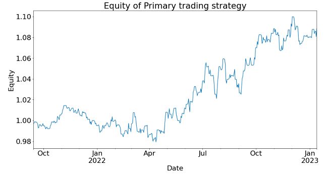
Figure

2: Equity curve of Primary trading strategy in out-of-sample period

What is Corrective AI?

Suppose
we have a trading model (like the Primary trading strategy described above) for setting the side of the bet (long or short). We just need to learn the size of that bet, which includes the possibility of no bet at all (zero sizes). This is a situation that practitioners face regularly. A machine learning algorithm (ML) can be trained to determine that. To emphasize, we do not want the ML algorithm to learn or predict the side, just to tell us what is the appropriate size.

We call this problem meta-labeling (Lopez de Prado, 2018) or Corrective AI (Chan, 2022) because we want to build a secondary ML model that learns how to use a primary trading model.

We train an ML algorithm to compute the “Probability of Profit” (PoP) for the next minute-bar. If the PoP is greater than 0.5, we will set the bet size to 1; otherwise we will set it to 0. In other words, we adopt the step function as the bet sizing function that takes PoP as an input and gives the bet size as an
output, with the threshold set at 0.5.  This bet sizing function decides whether to take the bet or pass, a
purely binary prediction.

The training period was from 2019-01-01 to 2021-09-30 while the out-of-sample test period was from 2021-10-01 to 2023-01-15, consistent with the out-of-sample period we reported for the Primary trading strategy. The model used to train ML algorithm was done using the predictnow.ai Corrective AI (CAI) API, with more than a hundred pre-engineered input features (predictors). The underlying learning algorithm is a gradient-boosting decision tree.

After applying Corrective AI, the Sharpe Ratio of the strategy in this period is 1.29  (an increase of 0.41), with average annual returns of 4.1% (an increase of 0.6%)  and a maximum drawdown of -1.9%
(a decrease of 1.6%). The alpha of the strategy is significantly improved.

The equity curve of the Corrective AI filtered secondary model signal can be seen in the figure below.

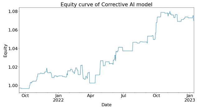
Figure
3: Equity curve of Corrective AI model  in out-of-sample period

Features used to train the Corrective AI model include technical indicators generated from indices, equities, futures, and options markets. Many of these features were created using Algoseek’s high-frequency futures and equities data. More discussions of these features can be found in (Nautiyal & Chan, 2021).

Conclusion:

By applying Corrective AI to the time-of-the-day Primary strategy, we were able to improve the Sharpe ratio and reduce drawdown during the out-of-sample backtest period. This aligns with observations made in the literature on meta-labeling for our primary strategies. The Corrective AI model's signal filtering capabilities do enhance performance in specific scenarios.

Acknowledgment

We are grateful to Chris Bartlett of Algoseek, who generously provided much of the high-frequency data for our feature engineering in our Corrective AI system. We also thank Pavan Dutt for his assistance with feature engineering and to Jai Sukumar for helping us use the Predictnow.ai CAI API. Finally, we express our appreciation to Erik MacDonald and Jessica Watson for their contributions in explaining this technology to Predictnow.ai’s clients

References

Breedon,
F., & Ranaldo, A. (2012, April 3). Intraday
Patterns in FX Returns and Order Flow. https://ssrn.com/abstract=2099321

Chan,
E. (2022, June 9). What is Corrective AI?
PredictNow.ai. Retrieved February 23, 2023, from
https://predictnow.ai/what-is-corrective-ai/

Lopez
de Prado, M. (2018). Advances in
Financial Machine Learning. Wiley.

Nautiyal,
A., & Chan, E. (2021). New Additions
to the PredictNow.ai Factor Zoo. PredictNow.ai. Retrieved February 28,
2023, from https://predictnow.ai/new-additions-to-the-predictnow-ai-factor-zoo/

Continue Reading

A New PositionBook Chart Type

It has been almost 6 months since I last posted, due to working on a house renovation. However, I have still been thinking about/working on stuff, particularly on analysis of open position ratios. I had tried using this data as features for machine learning, but my thinking has evolved somewhat and I have reduced my ambition/expectation for this type of data.

Before I get into this I'd like to mention Trader Dale (I have no affiliation with him) as I have recently been following his volume profile set-ups, a screenshot of one being shown below.

This shows recent Wednesday action in the EUR_GBP pair on a 30 minute chart. The flexible volume profile set-up Trader Dale describes is called a Volume Accumulation Set-up which occurs immediately prior to a big break (in this case up). The whole premise of this particular set-up is that the volume accumulation area will be future support, off of which price will bounce, as shown by the "hand drawn" lines. Below is shown my version of the above chart

with a bit of extra price action included. The horizontal yellow lines show the support area.

Now here is the same data, but in what I'm calling a PositionBook chart, which uses Oanda's Position Level data downloaded via their API.

The blue (red) horizontal lines show the levels at which traders are net long (short) in terms of positions actually entered/held. The brighter the colours the greater the difference between the longs/shorts. It is obvious that the volume accumulation set-up area is showing a net accumulation of long positions and this is an indication of the direction of the anticipated breakout long before it happens. The Trader Dale set-up presumes an accumulation of longs because of the resultant breakout direction and doesn't seem to provide an opportunity to participate in the breakout itself!

The next chart shows the action of the following day and a bit where the price does indeed come back down to the "support" area but doesn't result in an immediate bounce off the support level. The following order level chart perhaps shows why there was no bounce - the relative absence of open orders at that level.

The equivalent PositionBook chart, including a bit more price action,

shows that after price fails to bounce off the support level it does recover back into it and then even more long positions are accumulated (the darker blue shade) at the support level during the London open, again allowing one to position oneself for the ensuing rise during the London morning session, followed by another long accumulation during the New York opening session for a following leg up into the London close (the last vertical red line).

This purpose of this post is not to criticise the Trader Dale set-up but rather to highlight the potential value-add of these new PositionBook charts. They seem to hold promise for indicating price direction and I intend to continue investigating/improving them in the coming weeks.

More in due course.

Continue Reading

Simple Machine Learning Models on OrderBook/PositionBook Features

This post is about using OrderBook/PositionBook features as input to simple machine learning models after previous investigation into the relevance of such features. 

Due to the amount of training data available I decided to look only at a linear model and small neural networks (NN) with a single hidden layer with up to 6 hidden neurons. This choice was motivated by an academic paper I read online about linear models which stated that, as a lower bound, one should have at least 10 training examples for each parameter to be estimated. Other online reading about order flow imbalance (OFI) suggested there is a linear relationship between OFI and price movement. Use of limited size NNs would allow a small amount of non linearity in the relationship. For this investigation I used the Netlab toolbox and Octave. A plot of the learning curves of the classification models tested is shown below. The targets were binary 1/0 for price increases/decreases.

The blue lines show the average training error (y axis) and the red lines show the same average error metric on the held out cross validation data set for each tested model. The thickness of the lines represents the number of neurons in the single hidden layer of the NNs (the thicker the lines, the higher the number of hidden neurons). The horizontal green line shows the error of a generalized linear model (GLM) trained using iteratively reweighted least squares. It can be seen that NN models with 1 and 2 hidden neurons slightly outperform the GLM, with the 2 neuron model having the edge over the 1 neuron model. NN models with 3 or more hidden neurons over fit and underperform the GLM. The NN models were trained using Netlab's functions for Bayesian regularization over the parameters.

Looking at these results it would seem that a 2 neuron NN would be the best choice; however the error differences between the 1 and 2 neuron NNs and GLM are small enough to anticipate that the final classifications (with a basic greater/less than a 0.5 logistic threshold value for long/short) would perhaps be almost identical. 

Investigations into this will be the subject of my next post. 

The code box below gives the working Octave code for the above.

## load data
##training_data = dlmread( 'raw_netlab_training_features' ) ;
##cv_data = dlmread( 'raw_netlab_cv_features' ) ;
training_data = dlmread( 'netlab_training_features_svd' ) ;
cv_data = dlmread( 'netlab_cv_features_svd' ) ;
training_targets = dlmread( 'netlab_training_targets' ) ;
cv_targets = dlmread( 'netlab_cv_targets' ) ;

kk_loop_record = zeros( 30 , 7 ) ;

for kk = 1 : 30
  
## first train a glm model as a base comparison
input_dim = size( training_data , 2 ) ; ## Number of inputs.

net_lin = glm( input_dim , 1 , 'logistic' ) ; ## Create a generalized linear model structure.
options = foptions ; ## Sets default parameters for optimisation routines, for compatibility with MATLAB's foptions()
options(1) = 1 ;  ## change default value
##	OPTIONS(1) is set to 1 to display error values during training. If
##	OPTIONS(1) is set to 0, then only warning messages are displayed.  If
##	OPTIONS(1) is -1, then nothing is displayed.
options(14) = 5 ; ## change default value
##	OPTIONS(14) is the maximum number of iterations for the IRLS
##	algorithm;  default 100.
net_lin = glmtrain( net_lin , options , training_data , training_targets ) ;

## test on cv_data
glm_out = glmfwd( net_lin , cv_data ) ;
## cross-entrophy loss
glm_out_loss = -mean( cv_targets .* log( glm_out )  .+ ( 1 .- cv_targets ) .* log( 1 .- glm_out ) ) ;

kk_loop_record( kk , 7 ) = glm_out_loss ;

## now train an mlp
## Set up vector of options for the optimiser.
nouter = 30 ; ## Number of outer loops.
ninner = 2 ;	## Number of innter loops.
options = foptions ; ## Default options vector.
options( 1 ) = 1 ;	## This provides display of error values.
options( 2 ) = 1.0e-5 ; ## Absolute precision for weights.
options( 3 ) = 1.0e-5 ; ## Precision for objective function.
options( 14 ) = 100 ; ## Number of training cycles in inner loop.

training_learning_curve = zeros( nouter , 6 ) ; 
cv_learning_curve = zeros( nouter , 6 ) ;

for jj = 1 : 6

## Set up network parameters.
nin = size( training_data , 2 ) ; ## Number of inputs.
nhidden = jj ;	## Number of hidden units.
nout = 1 ; ## Number of outputs.
alpha = 0.01 ; ## Initial prior hyperparameter.
aw1 = 0.01 ;
ab1 = 0.01 ;
aw2 = 0.01 ;
ab2 = 0.01 ;

## Create and initialize network weight vector.
prior = mlpprior(nin , nhidden , nout , aw1 , ab1 , aw2 , ab2 ) ;
net = mlp( nin , nhidden , nout , 'logistic' , prior ) ;

## Train using scaled conjugate gradients, re-estimating alpha and beta.
for ii = 1 : nouter
  ## train net
  net = netopt( net , options , training_data , training_targets , 'scg' ) ;
  
  train_out = mlpfwd( net , training_data ) ;
  ## get train error
  ## mse
  ##training_learning_curve( ii ) = mean( ( training_targets .- train_out ).^2 ) ;
  
  ## cross entropy loss
  training_learning_curve( ii , jj ) = -mean( training_targets .* log( train_out )  .+ ( 1 .- training_targets ) .* log( 1 .- train_out ) ) ; 

  cv_out = mlpfwd( net , cv_data ) ;
  ## get cv error
  ## mse
  ##cv_learning_curve( ii ) = mean( ( cv_targets .- cv_out ).^2 ) ;
  
  ## cross entropy loss
  cv_learning_curve( ii , jj ) = -mean( cv_targets .* log( cv_out )  .+ ( 1 .- cv_targets ) .* log( 1 .- cv_out ) ) ; 
  
  ## now update hyperparameters based on evidence
  [ net , gamma ] = evidence( net , training_data , training_targets , ninner ) ;
  
##  fprintf( 1 , '\nRe-estimation cycle ##d:\n' , ii ) ;
##  disp( [ '  alpha = ' , num2str( net.alpha' ) ] ) ;
##  fprintf( 1 , '  gamma =  %8.5f\n\n' , gamma ) ;
##  disp(' ')
##  disp('Press any key to continue.')
  ##pause;
endfor ## ii loop

endfor ## jj loop

kk_loop_record( kk , 1 : 6 ) = cv_learning_curve( end , : ) ;

endfor ## kk loop

plot( training_learning_curve(:,1) , 'b' , 'linewidth' , 1 , cv_learning_curve(:,1) , 'r' , 'linewidth' , 1 , ...
training_learning_curve(:,2) , 'b' , 'linewidth' , 2 , cv_learning_curve(:,2) , 'r' , 'linewidth' , 2 , ...
training_learning_curve(:,3) , 'b' , 'linewidth' , 3 , cv_learning_curve(:,3) , 'r' , 'linewidth' , 3 , ...
training_learning_curve(:,4) , 'b' , 'linewidth' , 4 , cv_learning_curve(:,4) , 'r' , 'linewidth' , 4 , ...
training_learning_curve(:,5) , 'b' , 'linewidth' , 5 , cv_learning_curve(:,5) , 'r' , 'linewidth' , 5 , ...
training_learning_curve(:,6) , 'b' , 'linewidth' , 6 , cv_learning_curve(:,6) , 'r' , 'linewidth' , 6 , ...
ones( size( training_learning_curve , 1 ) , 1 ).*glm_out_loss , 'g' , 'linewidth', 2 ) ;

##  >> mean(kk_loop_record)
##  ans =
##
##     0.6928   0.6927   0.7261   0.7509   0.7821   0.8112   0.6990

##  >> std(kk_loop_record)
##  ans =
##
##     8.5241e-06   7.2869e-06   1.2999e-02   1.5285e-02   2.5769e-02   2.6844e-02   2.2584e-16

Continue Reading

OrderBook and PositionBook Features

In my previous post I talked about how I planned to use constrained optimization to create features from Oanda's OrderBook and PositionBook data, which can be downloaded via their API. In addition to this I have also created a set of features based on the idea of Order Flow Imbalance (OFI), a nice exposition of which is given in this blog post along with a numerical example of how to calculate OFI. Of course Oanda's OrderBook/PositionBook data is not exactly the same as a conventional limit order book, but I thought they are similar enough to investigate using OFI on them. The result of these investigations is shown in the animated GIF below.

This shows the output from using the R Boruta package to check for the feature relevance of OFI levels to a depth of 20 of both the OrderBook and PositionBook to classify the sign of the log return of price over the periods detailed below following an OrderBook/PositionBook update (the granularity at which the OrderBook/PositionBook data can be updated is 20 minutes):

• 20 minutes
• 40 minutes
• 60 minutes
• the 20 minutes starting 20 minutes in the future
• the 20 minutes starting 40 minutes in the future

for both the OrderBook and PositionBook, giving a total of 10 separate images/results in the above GIF.

 

Observant readers may notice that in the GIF there are 42 features being checked, but only an OFI depth of 20. The reason for this is that the data contain information about buys/sell orders and long/short positions both above and below the current price, so what I did was calculate OFI for:

• buy orders above price vs sell orders below price
• sell orders above price vs buy orders below price
• long positions above price vs short positions below price
• short positions above price vs long positions below price 

As can be seen, almost all features are deemed to be relevant with the exception of 3 OFI levels rejected (red candles) and 2 deemed tentative (yellow candles).

It is my intention to use these features in a machine learning model to classify the probability of future market direction over the time frames mentioned above. 

More in due course.

Continue Reading

A Possible, New Positionbook Indicator?

In my previous post I ended with saying that I would post about some sort of "sentiment indicator" if, and only if, I had something positive to say about my progress on this work. This post is the first on this subject.

The indicator I'm working on is based on the open position ratios data that is available via the Oanda api. For the uninitiated, this data gives the percentage of traders holding long and short positions, and at what price levels, in 14 selected forex pairs and also gold and silver. The data is updated every 20 minutes. I have long felt that there must be some value hidden in this data but the problem is how to extract it.

What I've done is take the percentage values from the (usually) hundreds of separate price levels and sum and normalise them over three defined ranges - levels above/below the high/low of each 20 minute period and the level(s) that span the price range of this period. This is done separately for long and short positions to give a total of 6 percentage figures that sum to 100%. Conceptually, this can be thought of as attaching to the open and close of a 20 minute OHLC bar the 6 percentage position values that were in force at the open and close respectively. The problem is to try and infer the actual, net changes in positions that have taken place over the time period this 20 minute bar was forming. In this way I am trying, if you like, to create a sort of  "skin in the game" indicator as opposed to an indicator derived from order book data, which could be said to be based on traders' current (changeable) intentions as expressed by their open orders and which are subject to shenanigans such as spoofing.

The methodology I've decided on to realise the above is constrained optimization using Octave's fmincon function. The objective function is simply:

    denom = X' * old_pb_net_pos ;

    J = mean( ( new_pb_net_pos .- ( ( X .* old_pb_net_pos ) ./ denom ) ).^2 ) ;

for a multiplicative position value change model where:

• X is a vector of constants that are to be optimised
• old_pb_net_pos is a vector of the 6 percentage values at the open
• new_pb_net_pos is a vector of the 6 percentage values at the close

This is a constrained model because percentage position values at price levels outside the bar range cannot actually increase as a result of trades that take place within the bar range, so the X values for these levels are necessarily constrained to a maximum value of 1 (implying no real, absolute change at these levels). Similarly, all X values must be greater than zero (a zero value would imply a mass exit of all positions at this level, which never actually happens).

The net result of the above is an optimised X vector consisting of multiplicative constants that are multiplied with old_pb_net_pos to achieve new_pb_net_pos according to the logic exemplified in the above objective function. It is these optimised X values from which the underlying, real changes in positions will be inferred and features created. More on this in my next post.

 

Continue Reading

Matrix Profile and Weakly Labelled Data - 2nd and Final Update

It has been over three months since my last post, which was intended to be the first in a series of posts on the subject of the title of this post. However, it turned out that the results of my work were underwhelming and so I decided to stop flogging a dead horse and move onto other things. I still have some ideas for using Matrix Profile, but not for the above. These ideas may be the subject of a future blog post.

I subsequently looked at plotting order levels using the data that is available via the Oanda API and I have come up with Octave code to render plots such as this:

where the brighter yellow stripes show ranges where there is an accumulation of sell/buy orders above/below price. These can be interpreted as support/resistance areas. It is normally my practice to post my Octave code, but the code for this plot is quite idiosyncratic and depends very much on the way I have chosen to store the underlying data downloaded from Oanda. As such, I don't think it would be helpful to readers and so I am not posting the code. That said, if there is actually a demand I am more than happy to make it available in a future blog post.

Having done this, it seemed natural to extend it to Open Position Ratios which are also available via the Oanda API. Plotting these levels renders plots that are similar to the plot shown above, but show levels where open long/short positions instead of open orders are accumulated. Although such plots are visually informative, I prefer something more objective, and so for the last few weeks I have been working on using the open position ratios data to construct some sort of sentiment indicator that hopefully could give a heads up to future price movement direction. This is still very much a work in progress which I shall post about if there are noteworthy results.

More in due course.

Continue Reading

A Temporal Clustering Function

Recently a reader contacted me with a view to collaborating on some work regarding the Delta phenomenon but after a brief exchange of e-mails this seems to have petered out. However, for my part, the work I have done has opened a few new avenues of investigation and this post is about one of them.

One of the problems I set out to solve was clustering in the time domain, or temporal clustering as I call it. Take a time series and record the time of occurance of an event by setting to 1, in an otherwise zero filled 1-dimensional vector the same length as the original time series, the value of the vector at time index tx and repeat for all occurances of the event. In my case the event(s) I am interested in are local highs and lows in the time series. This vector is then "chopped" into segments representing distinct periods of time, e.g. 1 day, 1 week etc. and stacked into a matrix where each row is one complete period and the columns represent the same time in each period, e.g. the first column is the first hour of the trading week, the second column the second hour etc. Sum down the columns to get a final 1-dimensional vector of counts of the timing of events happening within each period over the entire time series data record. A chart of such is shown below.

The coloured vertical lines show the opening and closing times of the London and New York sessions (7am to 5pm in their respective local times) for one complete week at a 10 minute bar time scale, in this case for the GBP_USD forex pair. This is what I want to cluster.

The solution I have come up with is the Octave function in the code box below

## Copyright (C) 2020 dekalog
## 
## This program is free software: you can redistribute it and/or modify it
## under the terms of the GNU General Public License as published by
## the Free Software Foundation, either version 3 of the License, or
## (at your option) any later version.
## 
## This program is distributed in the hope that it will be useful, but
## WITHOUT ANY WARRANTY; without even the implied warranty of
## MERCHANTABILITY or FITNESS FOR A PARTICULAR PURPOSE.  See the
## GNU General Public License for more details.
## 
## You should have received a copy of the GNU General Public License
## along with this program.  If not, see
## .

## -*- texinfo -*- 
## @deftypefn {} {@var{centre_ix} =} blurred_maxshift_1d_linear (@var{train_vec}, @var{bandwidth})
##
## Clusters the 1 dimensional vector TRAIN_VEC using a "centred" sliding window of length  2 * BANDWIDTH + 1.
##
## Based on the idea of the Blurred Meanshift Algorithm.
##
## The "centre ix" value of the odd length sliding window is assigned to the
## maximum value ix of the sliding window. The centre_ix, if it is not the 
## maximum value, is then set to zero. A pass through the whole length of
## TRAIN_VEC is completed before any assignments are made.
##
## @seealso{}
## @end deftypefn

## Author: dekalog 
## Created: 2020-10-17

function new_train_vec = blurred_maxshift_1d_linear ( train_vec , bandwidth )

if ( nargin < 2 )
 bandwidth = 1 ;
endif

if ( numel( train_vec ) < 2 * bandwidth + 1 )
 error( 'Bandwidth too wide for length of train_vec.' ) ;
endif

length_train_vec = numel( train_vec ) ;
assigned_cluster_centre_ix = zeros( size( train_vec ) ) ;

## initialise the while condition variable
has_converged = 0 ;

while ( has_converged < 1 )
 
new_train_vec = zeros( size( train_vec ) ) ;

## do the beginning and end of train_vec first
[ ~ , ix ] = max( train_vec( 1 : 2 * bandwidth + 1 ) ) ;
new_train_vec( ix ) = sum( train_vec( 1 : bandwidth ) ) ;

[ ~ , ix ] = max( train_vec( end - 2 * bandwidth : end ) ) ;
new_train_vec( end - 2 * bandwidth - 1 + ix ) = sum( train_vec( end - bandwidth + 1 : end ) ) ;

for ii = 2 * bandwidth + 1 : numel( train_vec ) - bandwidth
 [ ~ , ix ] = max( train_vec( ii - bandwidth : ii + bandwidth ) ) ;
 new_train_vec( ii - bandwidth  - 1 + ix ) += train_vec( ii ) ; 
endfor

if ( sum( ( train_vec == new_train_vec ) ) == length_train_vec )
 has_converged = 1 ;
else
 train_vec = new_train_vec ;
endif

endwhile

endfunction

I have named the function "blurred_maxshift_1d_linear" as it is inspired by the "blurred" version of the Mean shift algorithm, operates on a 1-dimensional vector and is "linear" in that there is no periodic wrapping of the data within the function code. The two function inputs are the above type of data, obviously, and an integer parameter "bandwidth" which controls the size of a moving window over the data in which the data is shifted according to a maximum value, hence maxshift rather than meanshift. I won't discuss the code further as it is pretty straightforward.

A chart of a typical clustering solution is (bandwidth setting == 2)

where the black line is the original count data and red the clustering solution. The bandwidth setting in this case is approximately equivalent to clustering with a 50 minute moving window. 

The following heatmap chart is a stacked version of the above where the bandwidth parameter is varied from 1 to 10 inclusive upwards, with the original data being at the lowest level per pane.

The intensity reflects the counts at each time tx index per bandwidth setting. The difference between the panes is that in the upper pane the raw data is the function input per bandwidth setting, whilst the lower pane shows hierarchical clustering whereby the output of the function is used as the input to the next function call with the next higher bandwidth parameter setting.

More in due course.

Continue Reading